This vignette explores more thoroughly some aspects of our work that might be overlooked in the other vignettes or in our paper. In particular, we will
- Explain how we generate TAD boundaries for analyzing 10X Single Cell ATAC-seq data
- Demonstrate how our method works on data involving only independent sets of pairwise distances (see Section 4.1 of our paper)
- Provide a population genetics example of how to run our method from the terminal
If you’ve come here for the details, you’re in the right place 🙂
Generating Topologically Associating Domains for scATAC-seq Data Analysis
This Section supplements our Analysis of Single Cell ATAC-seq Data vignette.
What are Topologically Associating Domains (TADs)?
Adapted from two review papers, Dixon et al. (2016) appearing in Molecular Cell and Szabo et al. (2019) appearing in Science Advances.
To understand TADs, we must first understand how a eukaryotic genome organises itself in space. Scientists already proposed, more than one hundred years ago, that chromosomes in “resting” interphase nuclei (i.e., not undergoing division) exist as chromosome territories. The figure below shows the writing of the late 19th century German zoologist Theodor Boveri, in which he described the looping of chromosomes amongst other ideas he had about “chromosome individuality.”
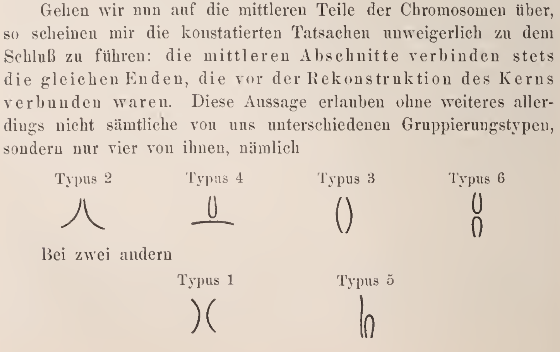
Obtained from Boveri (1909), available freely through the Biodiversity Heritage Library.
Similar to how chromosomes in the genome organise themselves territorially, each chromosome also has its own organisation, also referred to as chromosome folding. Within each chromosome are histone proteins, around which DNA is wound. Such compact DNA-histone complexes are called chromatin. The degree of packing of these complexes (i.e., how tightly compact or loose) is a dynamic process that depends on the stage of the cell cycle the cell is at.
Recent technologies have allowed the quantification of the folding patterns described above. Notably, chromosome conformation capture methods like Hi-C (Lieberman-Aiden et al., 2009) have uncovered folding patterns across different scales, measured through interactions (chromosomal contact frequencies). Here are two notable patterns:
- At large scales, chromosomes segregate into regions of preferential long-range interactions, forming two mutually excluded types of chromatin. These types correspond to gene-rich and active chromatin and to repressive chromatin.
- At a scale of tens to hundreds of kilobases, chromosomes fold into domains with preferential intradomain interactions compared to interdomain interactions. These contact domains are called TADs.
The figure below provides a visualisation of these folding patterns.
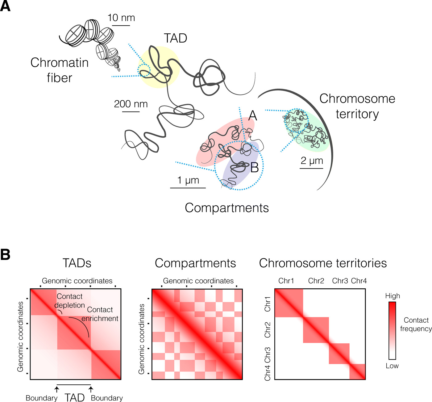
Hierarchical folding of the eukaryotic genome. (A) Many levels of chromatin folding, from the finest (DNA-histone association) to the coarsest (segregation of chromatin into active and repressed compartments). Each chromosome occupies its own territory within the nucleus. (B) Schematic representation of Hi-C maps at different genomic scales, reflecting different layers of high-order chromosome folding. Genomic coordinates are indicated along both axes. Figure reproduced from Szabo et al. (2019) under the Creative Commons Attribution NonCommercial (CC-BY-NC) license.
How do we find TADs?
Hi-C experiments measure contact frequencies across the genome, thus allowing scientists to identify TADs, which are the chromatin regions more frequently interacting within themselves than among each other. Before we discuss quantitative methods, it will be useful to see what our data looks like. Below, we load Hi-C contact maps obtained from human fibroblast cells (IMR90), as reported in Dixon et al. (2012). The reason our data is named hic_imr90_40 is that the Hi-C contact reads are binned at \(40,000\) bp resolution; this means that read counts are combined across genomic regions of length \(40,000\) bp.
## Load libraries
library(tidyverse)
require(HiTC) # install using Bioconductor if not installed
require(HiCDataHumanIMR90) # install using Bioconductor if not installed

## Load data
data(Dixon2012_IMR90)

## Preview data
# What type of object is it, and how large?
class(hic_imr90_40)
#> [1] "HTClist"
#> attr(,"package")
#> [1] "HiTC"
object.size(hic_imr90_40)
#> 1209797816 bytes

# What does a Hi-C map look like?
hic_imr90_40$chr1chr1@intdata[11:20,11:20]
#> 10 x 10 sparse Matrix of class "dsCMatrix"
#>
#> 11 . .  .    .   .  .  .   .   .    .
#> 12 . 2  .    .   .  .  .   .   .    .
#> 13 . . 22    2   .  .  .   .   .    1
#> 14 . .  2 2206 456  .  .   .   2    1
#> 15 . .  .  456  42  .  .   .   .    1
#> 16 . .  .    .   . 40  .   .   2    1
#> 17 . .  .    .   .  . 54   1   1    6
#> 18 . .  .    .   .  .  1 532  10    9
#> 19 . .  .    2   .  2  1  10 920   18
#> 20 . .  1    1   1  1  6   9  18 1240

# How are Hi-C features labeled?
head(hic_imr90_40$chr1chr1@xgi)
#> GRanges object with 6 ranges and 1 metadata column:
#>     seqnames        ranges strand |        name
#>        <Rle>     <IRanges>  <Rle> | <character>
#>   1     chr1       1-40000      * |           1
#>   2     chr1   40001-80000      * |           2
#>   3     chr1  80001-120000      * |           3
#>   4     chr1 120001-160000      * |           4
#>   5     chr1 160001-200000      * |           5
#>   6     chr1 200001-240000      * |           6
#>   -------
#>   seqinfo: 1 sequence from an unspecified genome; no seqlengths
For the rest of this vignette we restrict to Chromosomes 1 and 2, consistent with what we report in our paper. As part of pre-processing, we perform the following steps, as described in Sections 4 and 5.3 of the HiTC vignette.
- Binning contact frequency measurements into windows of size \(500,000\) bp (i.e., reducing the resolution from the original \(40,000\) bp)
- Normalising binned contact frequencies with Iterative Correction and Eigenvector decomposition (ICE)
## Restrict Hi-C data to chr1 and chr2
sset <- reduce(hic_imr90_40, chr=c("chr1", "chr2"))

## Bin contact frequencies
imr90_500 <- HTClist(mclapply(sset, binningC,
                              binsize=500000,
                              bin.adjust=FALSE,
                              method="sum",
                              step = 1))

## Perform ICE normalization
imr90_500_ICE <-  normICE(imr90_500, max_iter=1000) # converged at iteration 764

## Visualise transformed output of contact map
mapC(HTClist(imr90_500_ICE$chr1chr1), trim.range=.95,
     col.pos=c("white", "orange", "red", "black"))
We are now ready to identify TADs on our pre-processed dataset. As mentioned earlier, TADs are distinguished by intra-regional increase in interactions and inter-regional scarcity of interactions. We see this in the heat map above and can heuristically define TADs by inspection. However, to identify TADs in an automated fashion, we need systematic algorithms.
Here, we introduce two such systematic approaches. The first approach, called domainCaller, uses the Directionality Index (DI) to call TADs. Let the set of all \(40,000\) bp resolution counts be \(\mathscr{X}\). For each bin of contact frequencies \(x\in\mathscr{X}\), let \[\begin{equation*} \text{DI}(x) = \left(\frac{B(x) - A(x)}{|B(x) - A(x)|}\right) \left(\frac{(A(x) - E(x))^2}{E(x)} + \frac{(B(x) - E(x))^2}{E(x)}\right), \end{equation*}\] where
- \(A(x)\) is the number of reads that map from \(x\) to the upstream \(2\)Mb
- \(B(x)\) is the number of reads that map from \(x\) to the downstream \(2\)Mb
- \(E(x) = \frac{1}{2}(A(x) + B(x))\) is the expected number of reads under null of no directional bias
What domainCaller does is the following.
- Perform DI computation across all bins \(x\in\mathscr{X}\), obtaining a set of DIs \(\{\text{DI}(x):x\in \mathscr{X}\}\).
- Fit a hidden Markov model (HMM) to \(\{\text{DI}(x):x\in \mathscr{X}\}\).
- Use the inferred HMM states to define regions and classify them into TADs.
In Step 2 and Step 3, the HMM used is a three-state model (upstream bias, downstream bias, and no bias) with transition probabilities between successive bins. Details of this HMM can be found in Supplementary Figure 28 of Dixon et al. (2012).
One subtlety about TAD calling in Step 3: rather than inferring domains only, both domains and boundaries are inferred. A domain is initiated at the beginning of a single downstream biased state, and ends with the last state that is upstream biased. Regions between domains are classified as topological boundaries.
Fortunately, Hi-TC has made available the output of running domainCaller on our dataset. This is useful for us to gain intuition about what TADs look like, in preparation for the second approach we will introduce. Below, we load the domainCaller output.
## Inspect domainCaller output
tads_imr90@ranges
#> IRanges object with 2338 ranges and 0 metadata columns:
#>                start       end     width
#>            <integer> <integer> <integer>
#>      TAD-1    770138   1290137    520000
#>      TAD-2   1290138   1850140    560003
#>      TAD-3   1850141   2330140    480000
#>      TAD-4   2330141   3610140   1280000
#>      TAD-5   3770141   6077413   2307273
#>        ...       ...       ...       ...
#>   TAD-2334 146992309 148552096   1559788
#>   TAD-2335 148592096 149929342   1337247
#>   TAD-2336 149929343 151969344   2040002
#>   TAD-2337 152089345 152746806    657462
#>   TAD-2338 152786807 154946806   2160000

## Inspect number of TADs called in each chromosome
tads_imr90@seqnames
#> factor-Rle of length 2338 with 23 runs
#>   Lengths:   236   186   159   133   145   131 ...    63    58    34    27    86
#>   Values : chr1  chr2  chr3  chr4  chr5  chr6  ... chr19 chr20 chr21 chr22 chrX
#> Levels(23): chr1 chr2 chr3 chr4 chr5 chr6 ... chr18 chr19 chr20 chr21 chr22 chrX
The second approach to calling TADs is TopDom. Proposed by Shin et al. (2016), TopDom relies on a bin signal statistic to identify TADs. For each bin \(x\in\mathscr{X}\), let \[\begin{equation*} \text{binSignal}(x) = \frac{1}{w^2} \sum_{\ell=1}^w \sum_{m=1}^w \text{cont.freq}(U_x(\ell), U_x(m)), \end{equation*}\] where
- \(w\) is a window size parameter, to be fixed prior to identifying TAD boundaries
- \(U_x(\ell)\) and \(D_x(m)\) are bins located \(\ell\) indices upstream and \(m\) indices downstream of bin \(x\)
- \(\text{cont.freq}\) is the number of reads
As the formula suggests, \(\text{binSignal}\) computes the average contact frequency between upstream and downstream regions. See the Figure below for a visualisation.
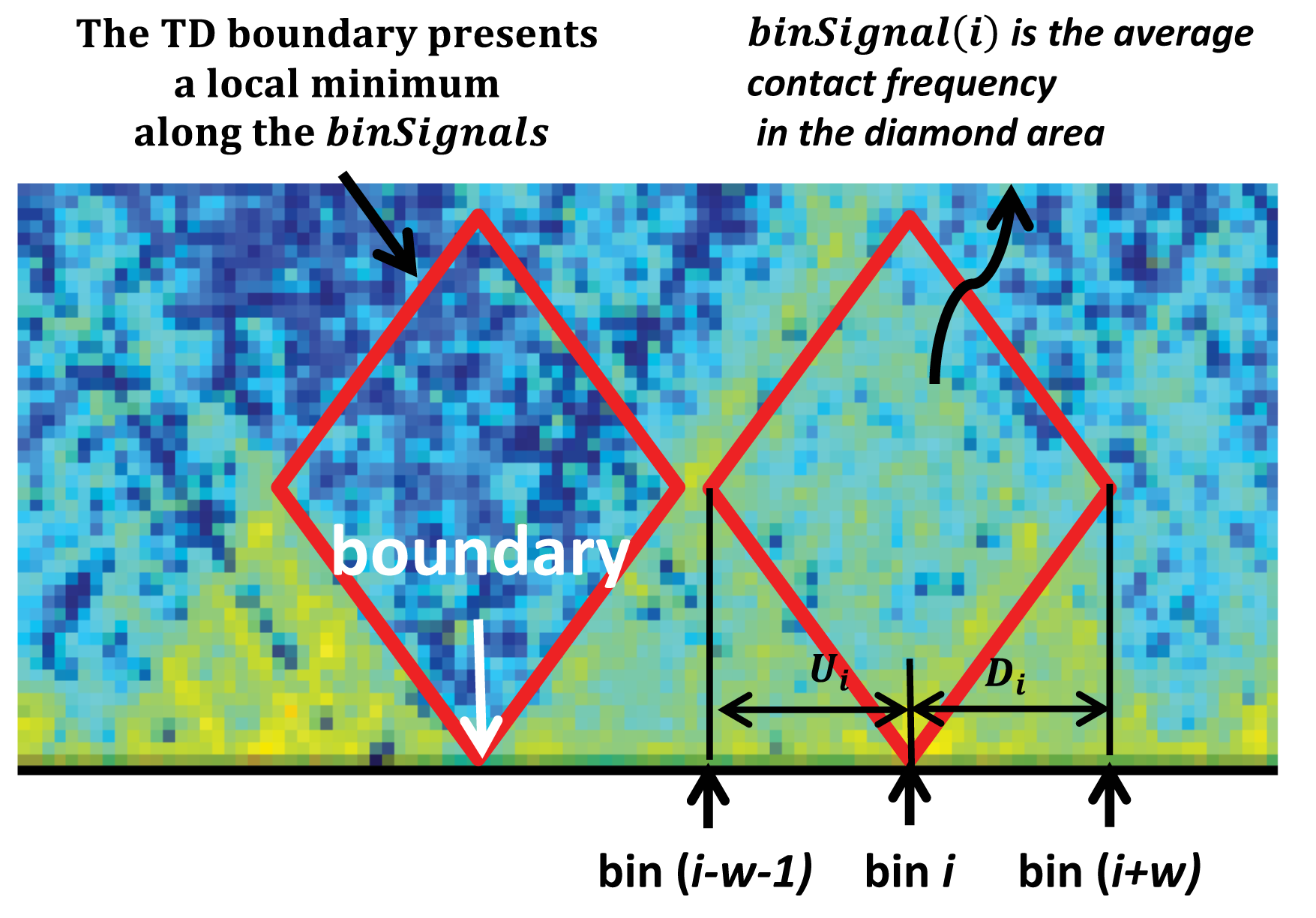
Denoting the bin \(x\) by its index \(i\), \(\text{binSignal}(i)\) is the average contact frequency between an upstream and a downstream chromatin region (\(U_i\) and \(D_i\)) in a window of size \(2w\) surrounding the bin. Its value is relatively high if bin \(i\) is located inside a TAD (red diamond), and reaches a local minimum at a TAD boundary. Figure adapted from Shin et al. (2016) under the Creative Commons Attribution NonCommercial (CC-BY-NC) license.
After computing bin signals for each bin, there is still a need to distinguish true local minima from false minima. To accomplish this, a sequential polygonal approximation technique is used to fit a smooth curve to the binsignal vs bin index graph. See the Figure below for a visualisation.
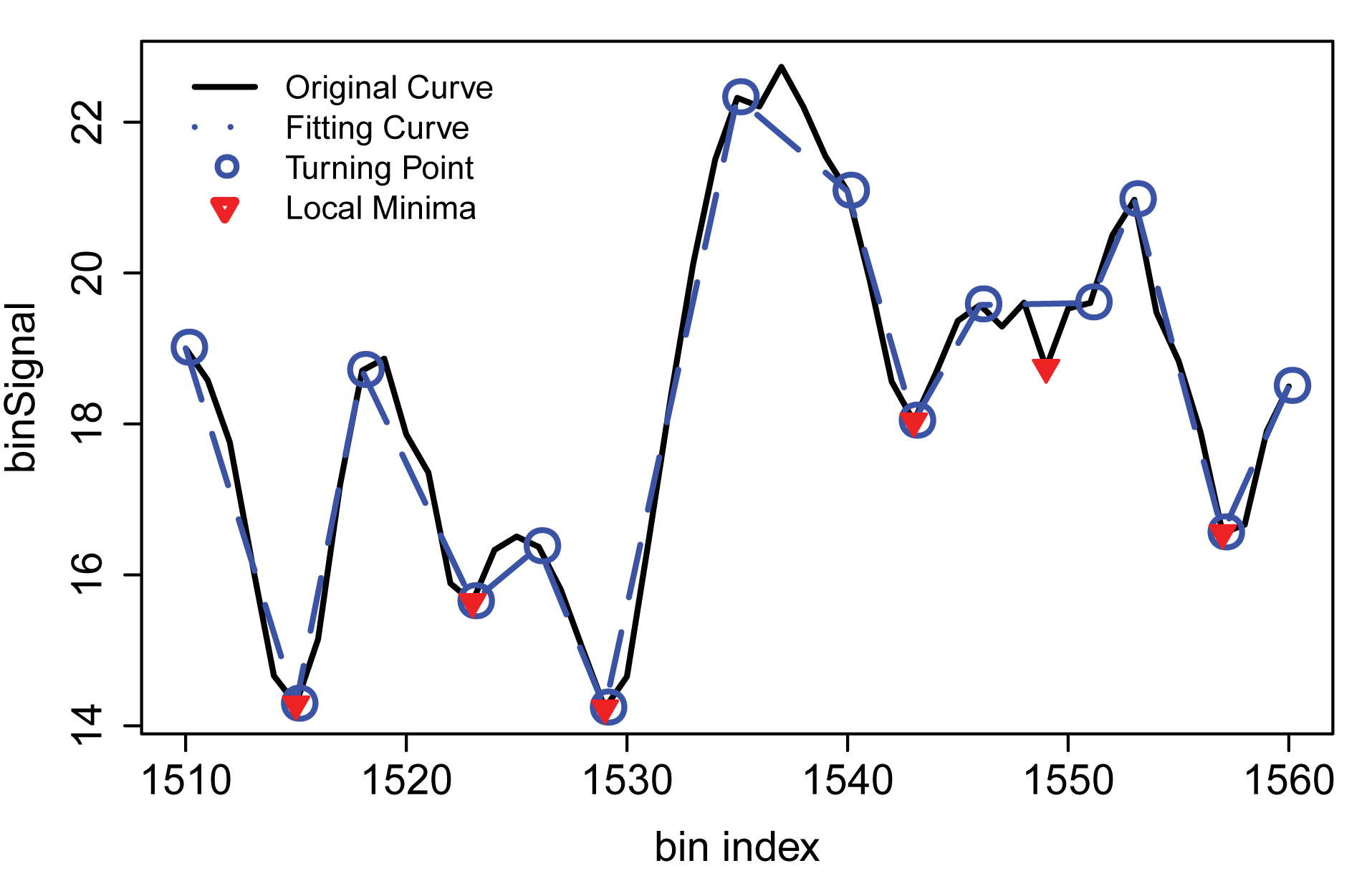
Turning points (blue circles) are identified in the original curve (black), and dominant local minima (red inverted triangles) are detected by fitting a piecewise linear curve (sequential polygonal approximation). Figure adapted from Shin et al. (2016) under the Creative Commons Attribution NonCommercial (CC-BY-NC) license.
Finally, to assign TAD boundaries, an additional Wilcoxon rank sum test is performed on the local minima selected.
Below, we demonstrate performing these steps on Chromosome 1 of the IMR90 dataset. We use a recent packaged version of TopDom, provided by Bengtsson et al. (2020).
## Load package
# install.packages("TopDom")
library(TopDom)

## Convert to format readable by TopDom::TopDom
# 1. Make imr90_500_ICE into N x (N + 3) dataframe
# We use the multiple assignment function, %<-%, provided by zeallot
library(zeallot)
df <- data.frame(chr = character(),
                 start = numeric(),
                 end = numeric())
for (i in 1:length(colnames(imr90_500_ICE$chr1chr1@intdata))) {
  c(chr_, start_, end_) %<-%
    strsplit(colnames(imr90_500_ICE$chr1chr1@intdata)[i], "\\:|\\-")[[1]]
  df <- rbind(df,
              data.frame(chr = chr_,
                         start = as.numeric(start_),
                         end = as.numeric(end_)))
}
topdom_input_500k <- cbind(df, as.matrix(imr90_500_ICE$chr1chr1@intdata))
rownames(topdom_input_500k) <- c()
colnames(topdom_input_500k) <- NULL
topdom_input_500k[,2] <- topdom_input_500k[,2] - 1

# What's the dimension of the newly formatted object?
dim(topdom_input_500k) # it's N x (N+3)
#> [1] 499 502

# What does it look like?
topdom_input_500k[1:6,1:10]
#>
#> 1 chr1       0  500000 0     0.00000     0.00000     0.0000     0.0000     0.00000
#> 2 chr1  500000 1000000 0 87119.73960  2201.44935   447.1085   141.7870    51.78014
#> 3 chr1 1000000 1500000 0  2201.44935 83144.23061  2036.0001   292.8696    89.12919
#> 4 chr1 1500000 2000000 0   447.10847  2036.00013 72933.3532  2894.1141   334.83724
#> 5 chr1 2000000 2500000 0   141.78698   292.86960  2894.1141 69802.3718  1759.64596
#> 6 chr1 2500000 3000000 0    51.78014    89.12919   334.8372  1759.6460 67023.35607
#>
#> 1    0.00000
#> 2   85.59758
#> 3   80.36681
#> 4  511.94974
#> 5 2209.51332
#> 6 4972.33528

# 2. Save as tab-delimited file
rel_dir <- "ex_data/scATAC-seq/"
#write.table(topdom_input_500k, file = paste0(rel_dir, "500k_topdom_input.tsv"),
#            row.names = FALSE,
#            col.names = FALSE,
#            sep="\t")

# 3. Load the file and find TADs with TopDom
# TopDom performs the steps described above
topdom_res <- TopDom::TopDom(paste0(rel_dir, "500k_topdom_input.tsv"), window.size = 5L)

# 4. View results
# What are the p-values?
head(topdom_res$binSignal)
#>   id  chr from.coord to.coord local.ext  mean.cf       pvalue
#> 1  1 chr1          0   500000      -0.5   0.0000 1.0000000000
#> 2  2 chr1     500000  1000000       0.0 292.7723 0.1791632334
#> 3  3 chr1    1000000  1500000      -1.0 225.5417 0.0002454393
#> 4  4 chr1    1500000  2000000       0.0 256.5692 0.0001367633
#> 5  5 chr1    2000000  2500000       0.0 311.2212 0.0009546703
#> 6  6 chr1    2500000  3000000       0.0 662.2543 0.1389660413

# Which blocks are classified as TADs by TopDom?
head(topdom_res$bed[which(topdom_res$bed$name ==  "domain"), ])
#>    chrom chromStart chromEnd   name
#> 6   chr1     500000  1500000 domain
#> 7   chr1    1500000  6500000 domain
#> 8   chr1    6500000 11000000 domain
#> 10  chr1   12000000 13000000 domain
#> 11  chr1   13500000 15500000 domain
#> 12  chr1   15500000 19500000 domain
To conclude this section, we look at the distribution of classification categories (not just TADs), as well as the distribution sizes (block lengths) of TADs.
## Look at distribution of classification results
kableExtra::kable(table(topdom_res$bed$name),
col.names = c("Category", "Count"))| Category | Count |
|---|---|
| boundary | 6 |
| domain | 44 |
| gap | 5 |
## Look at distribution of size of TADs
chr1_tads <- topdom_res$domain[which(topdom_res$domain$tag =="domain"), ]
kableExtra::kable(table(chr1_tads$size / 5e5),
col.names = c("Size (x 5e5 bases)", "Count"))| Size (x 5e5 bases) | Count |
|---|---|
| 2 | 4 |
| 4 | 2 |
| 5 | 6 |
| 6 | 3 |
| 7 | 4 |
| 8 | 5 |
| 9 | 6 |
| 10 | 4 |
| 11 | 1 |
| 15 | 1 |
| 16 | 1 |
| 18 | 1 |
| 20 | 1 |
| 21 | 1 |
| 24 | 1 |
| 26 | 2 |
| 29 | 1 |
Note we use these classified TADs to group our scATAC-seq features.
Test of Exchangeability Using Pairwise Distances
Our test of exchangeability works for settings where only pairwise distance data is available. Given a list of pairwise distances between \(N\) individuals, \(\{D_1,\ldots,D_B\}\), and assuming these distances are independent of one another, our test can determine whether the individuals making up the \(N\)-sample are exchangeable at a user-specified significance threshold (e.g., \(\alpha=0.05\)). (See Section of our paper.)
There are multiple practical scenarios well suited for such an approach.
- Loading the sample-by-feature matrix \(\mathbf{X}\) into memory is computationally unfeasible
- Only distance data is available owing to privacy issues
- Independent, large sets of features exist on different computers but need to be combined to form the sample-by-feature matrix \(\mathbf{X}\)
Below, we show how our method can be called on a list of distances, provided the features from which the pairwise distances are derived are mutually independent. Briefly, we have \(N=100\) individuals from whom we obtain \(50\) pairwise distance data, \(\{D_1,\ldots,D_{50}\}\). Each pairwise distance matrix \(D_b\) is computed from a block of \(10\) features, and we assume each block is independent of any other block.
## Simulation of list of distances
# Set seed for reproducibility
set.seed(2021)

# Generate data
N <- 100
num_rows <- choose(N,2)
B <- 50
dist_list <- list()
for (b in 1:B) {
  # Generate fake data
  if (b <= B/2) {
    fake_samples <- replicate(10, rbinom(N,1,0.5))
    fake_dist <- as.matrix(dist(fake_samples, method = "manhattan"))
  } else {
    fake_samples <- replicate(10, rnorm(N, sd = 10))
    fake_dist <- as.matrix(dist(fake_samples, method = "euclidean"))
  }

  # Add to list
  dist_list[[b]] <- fake_dist
}

# Clear garbage
gc()
#>             used   (Mb) gc trigger    (Mb) limit (Mb)   max used    (Mb)
#> Ncells  14068868  751.4   24208967  1292.9         NA   24208967  1292.9
#> Vcells 885563685 6756.4 1600378470 12210.0      16384 1600348721 12209.7
We now run our test of exchangeability on the list of distances.
## Apply test of exchangeability to simulated distance list
library(flintyR)
library(doParallel)
# Register parallel computation
registerDoParallel()

# Compute p-value
distDataPValue(dist_list) # should be >= 0.05
#> [1] 0.384
Running Our Test from Terminal
For users who prefer to run jobs from the terminal, we describe how to embed our test within “terminal-friendly” scripts. To facilitate our exposition, we use data from the 1000 Genomes (1KG) project (The 1000 Genomes Project Consortium, 2015). The 1KG data consists of individual genomes spanning 26 populations and 5 superpopulations. You may learn more about, and see some preliminary analyses of, the data here. If you are a geneticist, you probably already know more interesting analyses of this data.
The challenge here is that genomes are typically provided in VCF or BIM/BED/FAM or PGEN/PVAR/PSAM format. Moreover, they can be very large and thus cannot be loaded in memory.
Suppose our task at hand is to run a test of exchangeability on each 1KG population. There are millions of polymorphic variants, and we assume variants lying in different chromosomes are independent of one another. Since there are 22 autosomal chromosomes, this means that our features are grouped into 22 large blocks.
To accomplish our task, we perform the following steps.
- For each population, split the genome into the 22 autosomes.
- Per autosome:
- load it into R and construct its distance matrix
- remove the loaded autosome object from memory
- Run test of exchangeability on list of distance matrices. (See previous Section on this.)
Scripts that perform the steps above can be found in our Github repo, along with guidance on reproducing our results.
Preparing the population-level files
To obtain population-level files (BIM/BED/FAM) that can be fed into Step 1 above, we perform the following steps: (1) Download 1KG Phase 3 data (PGEN and PVAR) from here, see Merged dataset; (2) Filter to keep only variants that are in HapMap3 and UK Biobank; (3) Remove related individuals; (4) Filter to keep only biallelic SNPs with minor allele count at least \(1\) (this differs from usual filtering of alleles that satisfy MAF at least \(0.01\)); (5) Generate BED/BIM/FAM files for each population using population ID files. All of these steps are accomplished using PLINK2.Does Variant Filtering Affect Exchangeability?
Just to demonstrate a concrete implementation of the embedding approach and the scripts prepared above, we report \(p\)-values obtained by running our test on two versions of the 1KG data differing in the variants included.
- (Rare variants included, as described in Preparing the population-level files above) All biallelic variants that have minor allele count (MAC) at least \(1\) in the 1KG dataset are included.
- (Common variants only, as seen here and provided by the
read_1000Gfunction of the bigsnpr package) Only biallelic variants that have minor allele frequency at least \(0.01\) in the 1KG dataset are included.
Note that the analysis for the first scenario is as described in our Github repo.
We find that when using only common variants, all populations, except for the Yoruban population in Nigeria, are non-exchangeable at \(\alpha=0.05\) level. However, when additional rare variants are included, all populations are non-exchangeable at \(\alpha=0.05\).
## Print table summarising results
kableExtra::kable(data.table::fread("exchangeability_results.txt"))| POP | DESC | MAF1e-2 | MAC1 |
|---|---|---|---|
| GBR | British in England and Scotland | 0.00 | 0.000 |
| FIN | Finnish in Finland | 0.00 | 0.000 |
| CHS | Southern Han Chinese, China | 0.00 | 0.000 |
| PUR | Puerto Rican in Puerto Rico | 0.00 | 0.000 |
| CDX | Chinese Dai in Xishuangbanna, China | 0.00 | 0.000 |
| CLM | Colombian in Medellin, Colombia | 0.00 | 0.000 |
| IBS | Iberian populations in Spain | 0.00 | 0.000 |
| PEL | Peruvian in Lima, Peru | 0.00 | 0.000 |
| PJL | Punjabi in Lahore,Pakistan | 0.00 | 0.000 |
| KHV | Kinh in Ho Chi Minh City, Vietnam | 0.00 | 0.000 |
| ACB | African Caribbean in Barbados | 0.00 | 0.000 |
| GWD | Gambian in Western Division, The Gambia | 0.00 | 0.000 |
| ESN | Esan in Nigeria | 0.00 | 0.000 |
| BEB | Bengali in Bangladesh | 0.00 | 0.000 |
| MSL | Mende in Sierra Leone | 0.00 | 0.000 |
| STU | Sri Lankan Tamil in the UK | 0.00 | 0.000 |
| ITU | Indian Telugu in the UK | 0.00 | 0.000 |
| CEU | Utah residents with Northern and Western European ancestry | 0.00 | 0.000 |
| YRI | Yoruba in Ibadan, Nigeria | 0.07 | 0.022 |
| CHB | Han Chinese in Bejing, China | 0.00 | 0.000 |
| JPT | Japanese in Tokyo, Japan | 0.00 | 0.000 |
| LWK | Luhya in Webuye, Kenya | 0.00 | 0.000 |
| ASW | African Ancestry in Southwest US | 0.00 | 0.000 |
| MXL | Mexican Ancestry in Los Angeles, California | 0.00 | 0.000 |
| TSI | Toscani in Italy | 0.00 | 0.000 |
| GIH | Gujarati Indian in Houston,TX | 0.00 | 0.000 |
Thus, our test shows that most populations in the 1KG dataset are non-exchangeable, assuming variants lying in different chromosomes are independent of one another. In the only exception of the Yoruban population (YRI), we find that if only common variants are considered, then the individuals are exchangeable. However, once rare variants are included the individuals lose exchangeability. This observation is consistent with the importance of rare variants capturing recent demographic history, a point acknowledged by population geneticists (Zaidi and Mathieson, 2021).